Overview and History
The idea of generating Spice simulation models for vacuum tube circuits draws a lot of appeal to researchers who understand the limitations of the highly approximative classic theory. Unfortunately most of the techniques currently used to model vacuum tube devices fail to comply with the accepted practices of device modeling in several basic ways. First, the models are generally based on theoretical considerations instead of properly measured and averaged device transfer data; second, the models only address the output port current function and so provide an incomplete functional description of the device; thirdly, the models are fixed in the sense that one cannot readily alter them for customized match.
Early VT Spice models [1,2] are strongly based on assumptions made in tube circuit theory which were primarily intended to provide analytically tractable equivalent device replacements for use in hand analysis. These assumptions are: (i) a 3/2-power based expression for plate current, and (ii) a zero or near-zero expression for grid current. The 3/2-power law is derived from a one-dimensional representations of the tube's conduction channel and does not mimic u-factor dependence on terminal voltages whereas the zero grid current assumption represents the view of an idealized voltage sensing circuit and does not hold in large-signal situations. More recent modeling efforts [3,4] either introduce variant forms of the plate current expression or build on it to derive a more accurate match to unspecified data.
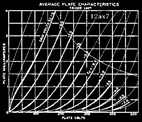
In order to generate device models useful for accurate Transient and AC simulations not only must absolute current levels match but they should also be close in the first order derivative (slope) of the transfer curves over the whole range. The divergence between the curvature of transfer curves of existing models and that of real devices has been mentioned previously [5], but here Fig. 1 shows precisely how poor Koren's 12ax7 model performs against corresponding RCA transfer data. Other researchers have also published comparative results based on Koren's model without intending to display descrepencies though their results strongly suggest otherwise [6].
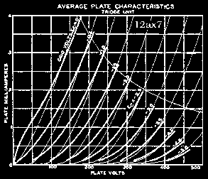
We see that the plate resistance in Koren's model, corresponding to the first derivative of the Ip(Vpc) curves, does not match well against RCA's in an area where typical load lines are known to lie. This is important because the poles and zeros of coupled circuits depend primarily on the dynamic properties of the active devices used, even more so in designs avoiding any kind of global feedback. It follows that this type of divergence in curve characteristics most likely would produce considerable numerical errors in circuit simulations and so cannot be trusted for exacting needs such as the design of an open-loop RIAA-compensated phono preamp.
A New Model For Vacuum Tube Triodes
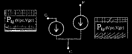
To solve such problems I propose a new model which is based on a complete definition of two-port networks and includes a freer algebraic expansion of the transfer characteristics which is derived from device data directly. The functional aspect of the model is covered by the principle which states that a two-port network is deemed completely specified over a given variable range if port currents can be determined in terms of both port voltages in that range. The model will be demonstrated for a 12ax7 vacuum tube triode though it can be applied to any other type of triode easily.
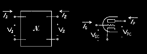
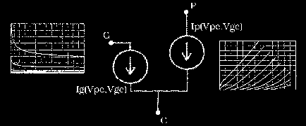
For a vacuum tube triode this means specifying Ip and Ig current functions in terms of both Vgc and Vpc voltage differences. This two-port formulation must hold over the device's intended range of application, one which is as wide as possible. This is of great relevance these days because researchers want to answer questions regarding the triode device behavior well into "full on" conditions, an area not well covered by past theories and models. Also, the model fit should be accurate over the main regions of application in absolute as well as incremental terms, that is, the first derivative of the approximation function should fit well against corresponding data derivative functions. When these three conditions are met we have obtained what should be considered a reasonable device substitute suitable for use in a simulation environment.
Reference Data
I use tube data provided by the RCA catalog [7] mainly because it is averaged and therefor lends itself well to a representative or generic model formulation. In other words, RCA data is taken as a reliable and universal guide for establishing model fit, though disagreement is possible in cases where strictness in regards to past measurement techniques is warranted. In an ideal case all individual brands and types of tubes should be tested, averaged and modeled, as is the case for transistors. When more accurate data becomes available, extracted with modern techniques, can official models be generated.
Because many of us are especially curious about tube behavior in the overload region the curves supplied by RCA need to be extended into the positive range of input voltages. Known to be erroneous for extracting complete sets of transfer curves, I use the grid shift technique on a GE 12ax7 to mark out two extra Ip(Vpc) curves not provided by RCA. Though this may seem incongruent and peculiar to some it will do for purpose of demonstration. The model will therefore possess a reliability range covering -5 to +1 volts on the input port. Outside this range the model has little guarantee of reliability and so input voltage levels should be monitored, especially in transient and swept-source simulations. The data used in generating the model is vectorised from a random choice of point pairs lying on the curves.
Grid current specs are not available for this tube although they can be extracted on the bench with a considerable degree of error. And because grid current levels are known to vary by as much as two orders of magnitude from tube to tube in a same manufacturing lot there is no reason to be too fussy with this side of the data as long as it corresponds moderately well. I use 6v6 grid current specs and scale it down to values which I've measured with 12ax7 tubes on the bench. Though this data should be provided accurately by modern test facilities in creating official models, again it will suffice for purposes of demonstration.
Polynomial Interpolation
In the case of vacuum tube triodes both the grid and plate current functions exhibit transfer characteristics which make them ideal for polynomial interpolation; that is, both current function dependencies to Vpc are knee-less, unlike transistor and pentode devices, and their evolution from one constant input voltage curve to the next very is very gradual. These two simple traits can be exploited to derive a model based on a polynomial interpolation of the vectorised data set. The advantage of using polynomial function lies in their ability and freedom to approximate all continuous functions accurately whereas the space covered by 3/2-power based and many other fixed order functions is greatly limited in comparison and would exhibit limits on approximation ability. Because polynomial interpolation involves weaving through point pairs the data needs to be log-converted in order to avoid negative current values when approaching the x-axis.
With or without this logarithmic scale conversion the basic idea behind the use of polynomial interpolation remains the same. That is, each curve making up the transfer set has a set of point pairs by which a set of polynomial coefficients can be extracted; I use Matlab for this [8]. Note that the resulting set of coefficients depends on the original choice of point pairs taken from the curves (see Table 1). So for every Ip(Vpc) or Ig(Vpc) curve corresponds a group of coefficients which can be listed in tabular form against the input voltage Vgc.
Because we interpolate each data vector to the same order each time this gives a very specific meaning to the column values of Table 2. Namely, each column represents a functional relationship between a particular coefficient order and the input voltage variable Vgc. Because the columns are also in vectorised form we can interpolate their function polynomial once again to yield coefficient sets corresponding to each column.
K0 = 3.3101e-3 6.4276e-2 4.7240e-1 1.5643e+0 1.8661e+0 -2.8135e+0 1.9145e+0 -9.9158e+0 K1 = 1.3632e-3 1.8921e-2 1.0492e-1 2.6213e-1 -4.8578e-2 -8.3349e-1 3.2558e-2 9.5428e-1 K2 = -1.4882e-3 -2.0981e-2 -1.0960e-1 -2.4952e-1 -1.7040e-1 2.2391e-1 2.5192e-2 9.5766e-02 K3 = 3.4761e-4 4.2512e-3 1.7002e-2 2.4265e-2 3.1025e-2 7.5560e-2 -3.9657e-2 -6.6107e-2 K4 = -2.4359e-5 -2.4727e-4 -5.6853e-4 5.2888e-4 -1.9288e-3 -1.3258e-2 4.7989e-3 8.4148e-3
Because this last set of coefficients can be used to generate not only the previous set of coefficients, by expanding the polynomial expression at the values of input voltage Vgc corresponding to the data, but also those coefficients corresponding to voltages lying between voltage values chosen to represent the data with. Provided the order is chosen properly in the second interpolation we can produce a fill-in which follows along with the general progression in the coefficient values themselves. The ability of each interpolation function to cut through the first level coefficients in a well- behaved manner is depicted in Figure 4.
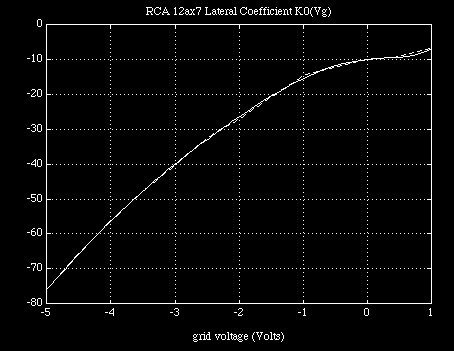
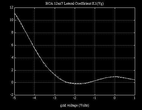
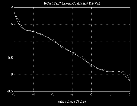
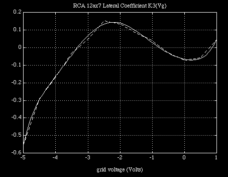
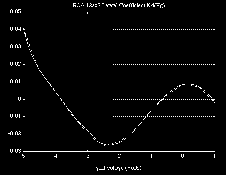
Clearly, if the interpolation at this second level weaves through the coefficient values of the first level interpolation, which is of a lower order and therefore requiring less numerical accuracy to reconstruct closely, then there is a good chance that the original data can be recovered from the last set of coefficients alone. In this case, with the log conversion and subsequent expansion taken into account, we can write a general form for the converted current function in a computationally economical polynomial expansion form in terms of terminal voltages as :
Ko(Vgc) +K1(Vgc) (Log(Vpc) +K2(Vgc) * (Log(Vpc) +K3(Vgc) * (Log(Vpc) +K4(Vgc) * Log(Vpc))))
In all cases the coefficient functions Ki(Vgc) is again a polynomial equation of the same form but without any Log terms since the only plate-to-cathode voltages are originally compressed.
One advantage provided by the log-scale conversion on the data is a reduction in transfer set curvature which allows for increased interpolation accuracy . However, this prevents us from reaching down all the way to Vpc=0v. So we establish an arbitrary low voltage minima (0.1v) on the second variable's domain and set by hand the data in the area of very low current and voltage as a means of guiding the polynomials appropriately through the important voltage regions. This is the only disadvantage to the model and one which can cause great pains in instances where the simulator rolls back the power supply voltage at the beginning of simulations.
For this reason initial values need to be set properly in many simulations or else failure to converge is almost guaranteed. The reason for this lies in the fact that the model now comprises two active ports with completely independent minds of its own unlike other models which have a passive front port and an active output port. Here, if one port sends its current function in the wrong direction too fast before the other port can make up its mind then circuit voltages will arise in which the model cannot recover itself and eventual convergence becomes impossible. To date there is no exact solution for this problem though it would have to involve low voltage data manipulation as some my own experiments have shown in the past.
Algorithm of Continuous, Monotonic and Reversible Transformations
The chain of continuously monotonic and reversible operations starting from the data, to the model and lastly to the output estimate is provided as follows:
(1) original data given as "functional" port current in terms of Vpc in vectorised form, each vector pair corresponding to a fixed value of input port voltage Vgc (2) log- log conversion on data to ensure non-negativity of interpolation, (3) polynomial coefficient extraction from data function vectors (4) separation of vector function into individual components (5) polynomial coefficient extraction of individual coefficient functions (6) coefficients of these polynomial functions stored in model, ( (7) coefficients used to generate any set of lower coefficient values continuously, i.e. for any value of Vgc (8) coefficients used to estimate the value of log-log current characteristic continuously for that value of input voltage Vgc; that is, for any value of Vpc (9) log of the output value calculated by expanding the polynomial function on the input value generates the estimate on current. (10) the value is exponentiated to reverse the log operation used in storing current data and so output estimate is obtained.
Provided the composition of all operations remains accurate, requiring each step to be accurate as well, we find the overall scheme approximates a reversible identity function on the original data set and therefore elsewhere provided the coefficient functions Ki(Vgc) are well behaved in the sense described above.
Pspice Subcircuit Model
The Pspice [9] subcircuit for the full model is listed below in Table 4, in it are found grid and plate current functions necessary for describing both functional and transfer characteristics of the device according to the general two-port formulation described above. Notice the repeated use of the Poly function which is a computationally efficient functional expression, a prime motivator for deriving the algorithm polynomially. Also, note the use of Log and Exp functions which are the next in level of computational complexity which are used only once each per netlist pass. Both these facts suggests that the model can run most efficiently though the netlist seems cumbersome compared to previous models which, in actual fact, make use of computationaly hefty subroutines.
Controlled voltage sources are used to implement the polynomial functions while a transconductance function converts the last operation to port current. Notice that the Pspice demo package does not penalize controlled source calls as much as, say, a diode subcircuit call. This means that larger circuits can be simulated in restricted platforms such as the demo version of Pspice. Dummy termination resistors on the inner polynomial controlled source circuits are provided in order to avoid what the simulator perceives as an inductor loop. Also, static parasitic capacitance values are provided as crude representatives although interpolation techniques similar to those used for terminal current could be used to model them as well based on the results of triode space-charge studies.
***************** p g c *************************************************** .subckt RCA12ax7 1 2 3 ************************* eGIogVpc 20 0 value={log(v(1,3))} rGlogVpc 20 0 1 eG0 10 0 poly(1) <2,3> -3.7694e+00 1.9947e+00 5.9432e-02 eG1 11 0 poly(1) <2,3> -3.2024e-02 -4.1443e-02 -4.8236e-03 eG2 12 0 poly(1) <2,3> 1.9127e-02 -1.2189e-02 -1.5526e-03 eG3 13 0 poly(1) <2,3> -1.1354e-02 4.9339e-03 6.1016e-04 rG0 10 0 1 rG1 11 0 1 rG2 12 0 1 rG3 13 0 1 gG 2 3 value={(exp(v(10)+v(20)*(v(11)+v(20)*(v(12)+v(20)*v(13)))))/170} * eP0 110 0 poly(1) <2,3> -9.9158e+0 1.9145e+0 -2.8135e+0 1.8661e+0 + 1.5643e+0 4.7240e-1 6.4276e-2 3.3101e-3 eP1 111 0 poly(1) <2,3> 9.5428e-1 3.2558e-2 -8.3349e-1 -4.8578e-2 + 2.6213e-1 1.0492e-1 1.8921e-2 1.3632e-3 eP2 112 0 poly(1) <2,3> 9.5766e-2 2.5192e-2 2.2391e-1 -1.7040e-1 + -2.4952e-1 -1.0960e-1 -2.0981e-2 -1.4882e-3 eP3 113 0 poly(1) <2,3> -6.6107e-2 -3.9657e-2 7.5560e-2 3.1025e-2 + 2.4265e-2 1.7002e-2 4.2512e-3 3.4761e-4 eP4 114 0 poly(1) <2,3> 8.4148e-3 4.7989e-3 -1.3258e-2 -1.9288e-3 + 5.2888e-4 -5.6853e-4 -2.4727e-4 -2.4359e-5 rP0 110 0 1 rP1 111 0 1 rP2 112 0 1 rP3 113 0 1 rP4 114 0 1 gP 1 3 value={(exp(v(110)+v(20)*(v(111)+v(20)*(v(112)+v(20)*(v(113)+v(20)*v(114))))))} Cgc 2 3 1.8p Cgp 2 1 1.7p Cpc 1 3 1.9p .ends
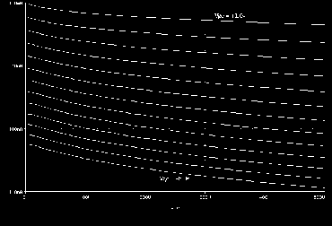
By comparing Spice output against original RCA data we can see that the fit is fairly accurate in both absolute and first order terms and should therefore allow us to determine more accurately important triode circuit characteristics such as small and large-signal distortion characteristics.
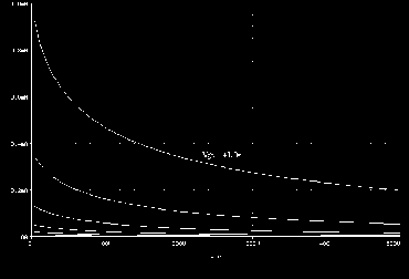
Grid current plot is shown in Figures 6a and 6b so that readers can be convinced of their validity. The grid current function is monotonic down to -5 volts which is as important for proper behavior as it is for the plate current function.
Large Signal Spice Simulations
The model presented here was derived primarily to accurately determine the non- linear drive and load properties of triode tube circuits and also for examining the effects of grid current and device transfer non-linearities in large-signal cascaded triode gain stage simulations. This is where wide-range device non-linear characteristics meet to produce some of the circuit behavior responsible for providing tube circuits with their signature feel.
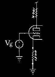
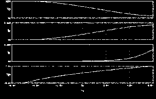
For example, the primary drive characteristics of a typical 100k/1.5k@300v gain stage employing a 12ax7 tube can be simulated to extract the exact wide-range circuit transfer function. This circuit transfer function can later be used to generate Fourier coefficient evolution against source amplitude to produce accurate harmonic distortion characteristics. A DC sweep is used to generate the various transfer functions present in the circuit against the circuit's input voltage sweep of -6v to +6v. Notice how the device's input port voltage Vgc varies against circuit input voltage Vg.
By simulating the front end of a cascaded triode circuit (Table 5), as seen in many amplifier circuits, we can highlight a property of triode tube circuits which is particularly relevant to guitarists. In particular we're interested in determining how grid current response changes (reflecting a dynamic response factor change) which seems to occur when the amp is full on compared to 90% by simulating the cascading of two gain stages.
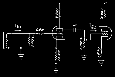
The test involves suddenly applying a 1KHz sine wave current to the grid of the first deliver energy to the circuit, and observe the waveform at the first plate as a function of second stage loading. By setting the input source to a large enough amplitude we overload the second stage so that the second grid circuit sources appreciable amounts of current relative to the plate circuit of the first stage.
In this test the potentiometer setting goes from full on to 90%. In the first case the v volume pot simply acts as a 1Meg load to ground with no series resistance between plate and grid of the two stages. In the second case, a one to nine reduction in grid voltage amplitude occurs because of the resistive voltage divider while introducing a 100kW resistor in the signal path. This resistive component attenuates grid current production and in fact has dropped by about 50%. Though a 10% voltage signal loss has occurred we see a 50% reduction grid current. This relative difference suggests a drastic increase in input circuit loading on the previous stage when the pot is turned full on. Though somewhat crude, this test lays a foundation for explaining why Fender Blackface amplifiers have a smoother, less distortive, response compared to the older Fender Tweed amps.
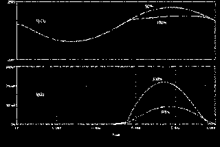
Further step transient simulations can show that, indeed, grid current plays an interesting role in establishing compressive effects. Other simulations have shown that plate transfer non-linearities together with grid current characteristics work together in the same direction towards establishing large-signal compression effects.
Cascaded gain stages with RCA 12ax7 spice model * Vsupply 99 0 300 * input pickup represented as ideal sinusoidal current source Iin 0 1 sin(0 1e-6 1000hz 0) *input resistor *low input 2 Rg1 1 2 68k *high input 1 *Rg1 1 2 34k *first gain stage Rg2 2 0 1Meg Rc1 3 0 1.5k Rp1 99 4 100k x1 4 2 3 RCA12ax7 Cs1 4 5 .02u * pot at 100% rotation Rvol1 5 6 1 Rvol2 6 0 1Meg * pot at 90% rotation *Rvol1 5 6 100k *Rvol2 6 0 900k *second gain stage *zero volt source used as 0W current monitor Vig2 6 96 0 x2 8 96 7 RCA12ax7 Rp2 99 8 100k Rc2 7 0 1.5k
*** insert 12ax7 tube model here
*initial conditions .ic v(2)=-0.570591 v(3)=1.4180 v(4)=230.526 v(5)=-0.570591 + v(6)=-0.570591 v(7)=1.4180 v(8)=230.526 *transient and output processor calls in pspice .tran 1e-6 1e-3 0 1e-6 .probe .end
------------- References
1. Dr. W. Marshall Leach, Jr., "SPICE Models for Vacuum Tube Amplifiers," JAES, Vol. 43, No. 3 (March 1995) pp. 117-126
2. S. Reynolds, "Vacuum-Tube Models for SPICE Simulations," GA 4/93, pp.17-23
3. N. Koren, "Improved VT Models for Spice Simulation," GA 5/96, pp. 18-27, 69
4. C. Rydel, "Tube Modeling," GA (Letters) 6/96, pp. 69-71
5. E. Pritchard, "Tube-Model Critique", GA (Letters) 1/96, pp. 54-57
6. J. Tolonen, "High-performance Tubed DAC Output Stage," GA 2/97, pp. 22-32
7. RCA Tube Manual, 1958
8. Matlab, Student Edition, The MathWorks, Inc. 1992
9. Pspice 6.0, MicroSim Corporation, 1994